Latency
We use the notation of the overview: a filter of finite duration \(T\) applied to a signal \(x(t)\) by the convolution of Impulse Response and Convolution. In a real-time stream, "latency" names more than one thing, and the kinds must be kept apart.
Kinds of latency
Definition: physical (timestamp) latency
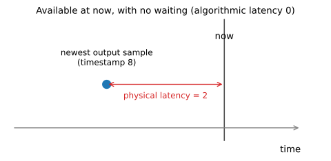
In a stream of timestamped samples produced in real time, the physical latency, or timestamp latency, is the difference between the reference time, now, and the timestamp carried by the most recent sample the stream has produced. It measures how far behind the present the stream's labeled time runs. It is a property of the channel and is read directly from the timestamps, independently of anything that consumes the stream.
Example: reading physical latency
If at now \(= 10\) the stream has just produced a sample labeled \(t = 8\), the physical latency is \(10 - 8 = 2\). The data is real and present; its timeline simply lags the present by two units.
Definition: algorithmic latency
The algorithmic latency of a processing stage is the wall-clock delay it adds before it can emit a given output, because it must first accumulate or wait for input. A stage with zero algorithmic latency emits each output as soon as the input that output depends on has arrived.
Example: look-ahead costs algorithmic latency
A stage that must see \(k\) samples beyond the current one before it can emit its output waits for those \(k\) samples to arrive, adding \(k\) samples of algorithmic latency. A stage that transforms each sample as it arrives adds none, even if it relabels the output's timestamp.
The two are independent. A filter's group delay shifts features in time; recording an earlier timestamp on the output, as described below, realigns a feature with its timestamp. In a real-time stream that realignment shows up as physical latency, but it need not add any algorithmic latency, since the values can be relabeled and passed on at once.
Choosing the timestamp
The output at time \(t\) draws on the input over the window \([t - T,\, t]\), and one must decide which instant of that window to record as the time of the output. This choice sets the physical latency; it changes no computed value, and it adds no algorithmic latency.
The window \([t - T,\, t]\) admits three natural timestamps, each suited to a different filter.
Example: three timestamps for one window
Label the output with the newest input time \(t\), the center \(t - T/2\), or the oldest \(t - T\):
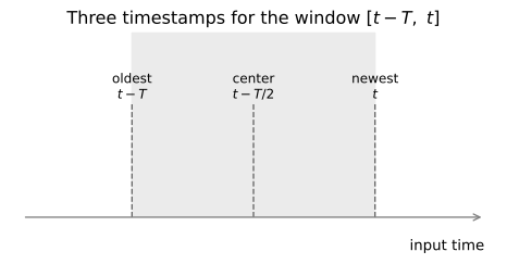
The newest time suits a filter whose energy lies at the front of its impulse response, a causal, minimum-phase filter. The center suits a symmetric, linear-phase filter, whose group delay is exactly \(T/2\). The oldest suits a filter whose energy lies at the back, an anti-causal filter.
The correct timestamp is the one under which a feature present in the input appears at its true time in the output, namely the labeling that offsets the output by the filter's group delay. An incorrect choice merely displaces the entire output stream in time.
This alignment is exact only when the group delay is the same at every frequency, which holds for a linear-phase filter and fixes the center timestamp \(t - T/2\). When the group delay varies with frequency, no single timestamp aligns every feature at once; the newest time \(t\) is then the natural choice, giving a causal output with the least physical latency.
In discrete time
With \(N\) taps the window spans the input indices \(n - (N-1)\) through \(n\), and the three timestamps are \(n\), \(n - (N-1)/2\), and \(n - (N-1)\). The linear-phase choice \((N-1)/2\) is the group delay of a symmetric filter.
Placing a unit impulse at index \(5\) and filtering with the symmetric filter \((1/4, 1/2, 1/4)\), whose group delay is one sample, puts the output peak at index \(6\); subtracting the group delay recovers the impulse's true position:
import numpy as np

x = np.zeros(11)
x[5] = 1.0
h = np.array([0.25, 0.5, 0.25])          # symmetric, group delay 1
y = np.convolve(x, h)
peak = int(np.argmax(y))
assert peak == 6
assert peak - (len(h) - 1) // 2 == 5
References
- Latency (engineering) (Wikipedia).
- Group delay and phase delay (Wikipedia).
- Causal filter (Wikipedia).